We often fly blind in the world of machine learning. Our model outputs an estimate for revenue from clicking on a certain ad, or the amount of time until a new edition of a book comes out, or how long it will take to drive a certain route. Typically these estimates are in the form of a single number with implicitly high confidence. Trusting these models can be foolish! Perhaps our models are high-tech con men -- Frank Abagnale reborn in the form of a deep neural net.
If we want to call ourselves "Data Scientists", perhaps it is time to behave like scientists do in other fields.
I didn't study a natural science (like astronomy or biology), but I did take a few physics classes with labs. One such lab required us to find the gravitational constant by dropping a metal ball from a variety of heights. During the experiment we were careful to record uncertainties in our measurements, and we propagated uncertainty through to our final estimate of the gravitational constant. If I had turned in a lab report claiming g = 9.12 m/s^2 (without any uncertainty estimate), I would have lost points.
Good scientific measurements come with uncertainty. A ruler or measuring tape is only so precise. When it comes to machine learning, though, this focus on uncertainty disappears.
For example, see this common formulation of the learning problem from the book Learning from Data [0] (no shade -- I love this book):
There is a target to be learned. It is unknown to us. We have examples generated by the target. The learning algorithm uses these examples to look for a hypothesis that approximates the target.
This unknown target function they call f: X -> Y (where X is the input/feature space and Y is the output/target space). The hypothesis approximating the target they denote as g: X -> Y (and, if our learning algorithm is successful, we can say g ≈ f).
In the case of regression, the output of our learning algorithm is a function which produces a continuous-valued output. But this output is a point estimate. It has no sense of uncertainty [1]!
Others have of course noted the importance of uncertainty estimation before me. One such person is José Hernández-Orallo (a professor at Polytechnic University of Valencia), whose paper Probabilistic reframing for cost-sensitive regression I found while researching class imbalance. I would be misrepresenting his work to claim this paper is solely about uncertainty/reliability estimation, but he describes some neat ideas worth exploring.
Rather than finding a function g: X -> Y approximating the true underlying function f, we could instead seek to find a probability density function h(y | x). In other words, a function to which we can still pass some features (x) but one describing a distribution instead of a point estimate. Because we are estimating a probability density function conditioned on the input features, this idea is called conditional density estimation.
To hear Hernández-Orallo tell it, many methods for conditional density estimation are suboptimal. The mean of the distributions they output is typically worse than a point estimate would have been. They are often slow. And in many cases, the distributions don't end up being multi-modal anyway. Thus, the paper asserts we can get by with a method to provide a normal (Gaussian) density function for most cases.
Normal distributions are parametrized by a mean and a standard deviation. Taking a point estimate (from any regression model) as the mean, we still need to determine the standard deviation. The paper describes a few different approaches for doing this (and is worth reading if you have the time). For the sake of this post, I'll focus on a technique called "univariate k-nearest comparison". A simple Python implementation follows:
def univariate_knearest_comparison(model, dataset, test_point, k=3):
    all_preds = model.predict(dataset)
    Q = zip(all_preds, dataset["Weight"].values)
    prediction = model.predict(test_point)
    neighbors = sorted(
        ((y_pred, y_true) for y_pred, y_true in Q),
        key=lambda t: np.abs(t[0] - prediction),
    )[:k]
    variance_estimate = (1 / k) * sum(
        (prediction - y_true) ** 2 for _, y_true in neighbors
    )
    return prediction[0], variance_estimate[0]
Hernández-Orallo describes this procedure as looking "for the closest estimations in the training set to the estimation for example x", then comparing "their true values with the estimation for x".
This technique is cool because it can be applied to any regression model. By using the training set (or a validation set) in this clever way, we can enrich any model with the ability to estimate uncertainty (thus gaining the second aspect of what we've been calling trustworthy models).
If you've not read previous posts in this series, we've been working with a dataset about fish. From their dimensions, we're trying to predict their weight. It's totally a toy/unrealistic problem, but it's pedagogically useful.
We'll start by training a linear model.
ct = ColumnTransformer([
    ('scale', StandardScaler(), ['Length1', 'Length2', 'Length3', 'Height', 'Width']),
    ('ohe', OneHotEncoder(), ['Species']),
])

pipe = make_pipeline(ct, lm.LinearRegression())
pipe.fit(fish, fish['Weight'])
Then, we'll run the univariate k-nearest comparison function from above.
new_fish = pd.DataFrame(
    [
        {
            "Species": "Bream",
            "Weight": -1,
            "Length1": 31.3,
            "Length2": 34,
            "Length3": 39.5,
            "Height": 15.1285,
            "Width": 5.5695,
        }
    ]
)

pred, var = univariate_knearest_comparison(pipe, fish, new_fish)
# (646.1153309725989, 4896.726887004621)
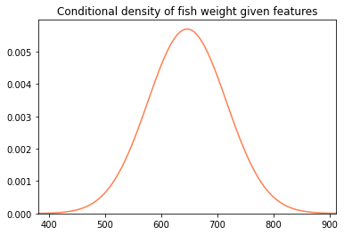
With our prediction and variance estimate in hand, we can draw a normal distribution.
import scipy.stats as st

def plot_normal(pred, var, color='coral', do_lims=True):
    width = np.sqrt(var) * 3.8
    x_min, x_max = pred - width, pred + width

    x = np.linspace(x_min, x_max, 100)

    y = st.norm.pdf(x, pred, np.sqrt(var))

    plt.plot(x, y, color=color)
    if do_lims:
        plt.xlim(x_min, x_max)

        ylo, yhi = plt.ylim()
        plt.ylim(0, yhi)

        plt.title('Conditional density of fish weight given features')

plot_normal(pred, var)
Here's a little graph with conditional density estimates for several different fish on it.
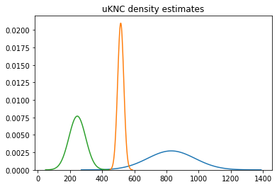
This is a strong step in the direction of being more scientific in our modeling efforts. We've examined a few methods for uncertainty estimation in this series, and we'll evaluate the quality of these techniques at a later date.
If you found this interesting, consider following me on Twitter.