We live in a world of imperfect information. When faced with a lack of data, we can make a guess. This guess could be far from the truth; it could be spot on. In Monte Carlo simulation, we repeatedly make guesses of some unknown value according to some distribution and are able to report on the results of that simulation to understand a little bit more about the unknown. While any one guess may be far from the truth, in aggregate those outliers don't have as much of an effect.
I ran into a situation where I was gathering some data with some level of imperfection. My stakeholder wanted to know what the impact of that imperfection on the important metrics would be. I could have made a guess, but instead I turned to the data. Initially, I thought to calculate the best case and worst case scenarios. This idea is useful in that it gives you a range on what you don't know, but it's also beneficial to know how likely each of those scenarios (and things in between) are. That's where Monte Carlo simulation comes in handy.
For the purposes of context, let's use a contrived example. Suppose I run a car dealership, and a major hail storm rolled through last weekend. Some of my cars suffer major damage and will incur a 10% loss in their value, some suffered minor damage incurring a 5% loss, and some suffered no damage at all. I don't have enough labor to survey every single one of my cars, but I do want to know how much money I can expect to lose. I randomly select 500 of my 1000 cars and see how bad the damage was.
Hypothetically, it's possible that the 500 cars I inspected were the only ones that happened to have been damaged by the hail (maybe the rest were safe in my 500-car warehouse). That would be the best case scenario, in which case I suffer only the loss on the cars I inspected. In the worst case scenario, every car I didn't inspect suffered major damage. For some random data I generate below, we know that the amount of damage done to the uninspected cars is somewhere between 0 and around $1.75 million dollars. This is a huge range of possibilities!
We see that looking at the best case and worst case gets us some bounds on how bad the damage could be, but we have no idea how probable each of these options are (let alone the probability of the values in the middle). To find out how bad the damage is likely to be, we can turn to Monte Carlo simulation.
First, let's randomly generate our inventory, then inspect half of our cars. While we know the value of each car, we
think of the damage_pct as an unknown value for the cars we do not inspect.
import pandas as pd
import numpy as np
import matplotlib.pyplot as plt

N_CARS = 1000
cars = pd.DataFrame({
    'value': np.random.normal(35000, 5000, size=N_CARS),
    'damage_pct': np.random.choice([-0.1, -0.05, 0], size=N_CARS, p=[0.1, 0.5, 0.4])
})

inspected_cars = cars.sample(cars.shape[0] // 2)
uninspected_cars = cars[~cars.index.isin(inspected_cars.index)]

damage_dist = (inspected_cars.groupby('damage_pct').count()
               / inspected_cars.shape[0]).rename(columns={'value': 'prob'})
We can see the distribution of damage_pct among the sampled cars is1:
| damage_pct | prob |
|---|---|
| -0.1 | 0.096 |
| -0.05 | 0.490 |
| 0.00 | 0.414 |
Because we inspected a random subset of the cars, a reasonable simplifying assumption is that the damage to the uninspected cars has the same distribution as that of the inspected cars. With that assumption, we can simulate the damage done to the uninspected cars like so:
def simulate_damage(damage_dist, uninspected_cars):
    damage_pct_guess = np.random.choice(damage_dist.index,
                                        size=uninspected_cars.shape[0],
                                        p=damage_dist.prob)
    return (damage_pct_guess * uninspected_cars.value).sum()

N_SIMULATIONS = 1000
simulated_damages = pd.Series([simulate_damage(damage_dist, uninspected_cars)
                               for _ in range(N_SIMULATIONS)])
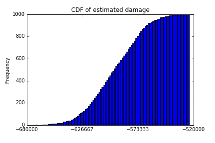
To make sense of the output of these 1000 simulations, we can calculate some descriptive statistics. It's also helpful to look at the CDF of the simulated damage.
print(simulated_damages.describe())
simulated_damages.plot(kind='hist', cumulative=True, bins=100,
                       title='CDF of estimated damage')
count      1000.000000
mean    -595662.074433
std       25097.417355
min     -671499.963571
25%     -613690.059583
50%     -595382.298010
75%     -576089.086686
max     -524043.037134
We can say that in half of our simulations, the damage was somewhere between $671,499.96 and $595,382.30. This range is about 4.3% the size of the range between the best and worst case scenarios.
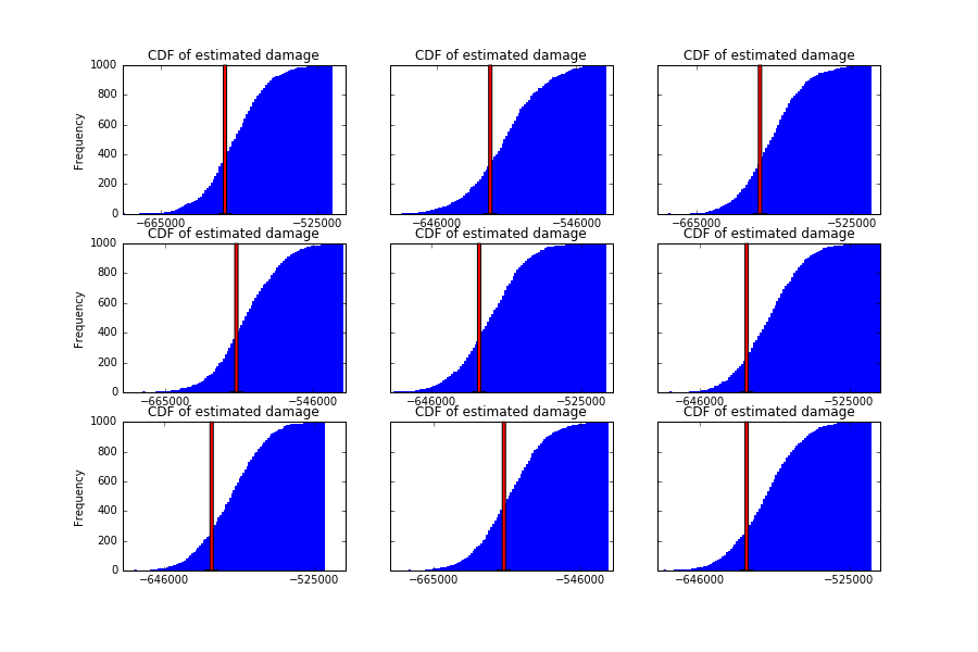
How'd we do? Because we made up the dataset, we can calculate the true value and put that number on the graph above:
true_damage = (uninspected_cars.value * uninspected_cars.damage_pct).sum()
bottom, top = plt.ylim()
plt.annotate('', xy=(true_damage, top), xycoords='data',
             xytext=(true_damage, bottom), textcoords='data'
             arrowprops=dict(facecolor='red', width=3, headlength=1))

In "reality", the true amount of damage done was $607,830.94, which just so happens to be in that window of 50% of our simulations.
We can run this experiment a few more times to see how this method fares:
The next time you're trying to reason about some unknown value, consider using Monte Carlo simulation to inform your decision-making process.
1: While the values for damage_pct look like numerical data, remember that they are representative of the three
categories of damage sustained (none, minor, or major).